
Field Notes Journal Entry
Looking for Structure in the Year
Moving from individual species models towards whole-community seasonal structure using feature extraction, similarity analysis, and ecological heatmaps
The earlier stages of the seasonal modelling work focused almost entirely on individual species.
The questions were fairly localised:
- Can a model reproduce the seasonal shape of a robin?
- Can a winter visitor model capture the structure of redwing records?
- Can flowering curves be represented mechanistically?
As the models developed, however, another possibility started to emerge.
If each species could be represented as a structured collection of seasonal features, could those features then be compared across the wider ecological community?
This post describes the first steps in exploring that idea.
From Models to Feature Sets
Once the individual model families became reasonably stable, the next stage was to extract a common set of ecological descriptors from the fitted results.
Each species is now represented as a feature set describing aspects of its seasonal behaviour, including:
- Seasonal timing
- Peak periods
- Seasonal width
- Persistence
- Suppression structure
- Occupancy behaviour
- Trait classifications
- Derived ecological metrics
These feature sets are assembled into a species feature matrix, allowing the modelling system to move from analysing single species in isolation towards comparing seasonal structure across the wider dataset.
At this stage, the feature matrix acts less like a biological taxonomy and more like a structured description of seasonal ecological behaviour.
Comparing Seasonal Structure
Once species are represented numerically, pairwise similarity comparisons become possible.
The similarity system combines several forms of comparison:
- Circular month handling for seasonal timing
- Normalised numeric distances
- Categorical matching
- Trait overlap scoring
The result is a similarity mapping describing how closely species resemble one another in terms of their seasonal ecological signal.
Importantly, similarity in this system should be interpreted primarily as similarity of seasonal ecological signal rather than direct biological relationship, taxonomic affinity, or causal ecological interaction.
That distinction matters.
A butterfly and a flowering plant may appear strongly related within the similarity space, not because they are biologically equivalent, but because they occupy similar regions of the seasonal year.
In practice, this often turns out to be surprisingly ecologically plausible.
Emerging Seasonal Neighbourhoods
The most interesting part of the process was not the similarity calculations themselves, but the structure that began to appear once the results were visualised.
To explore the relationships between species, the pairwise similarity matrix was rendered as a clustered heatmap.
Species with similar seasonal signatures are placed close together, producing visible neighbourhoods within the matrix.
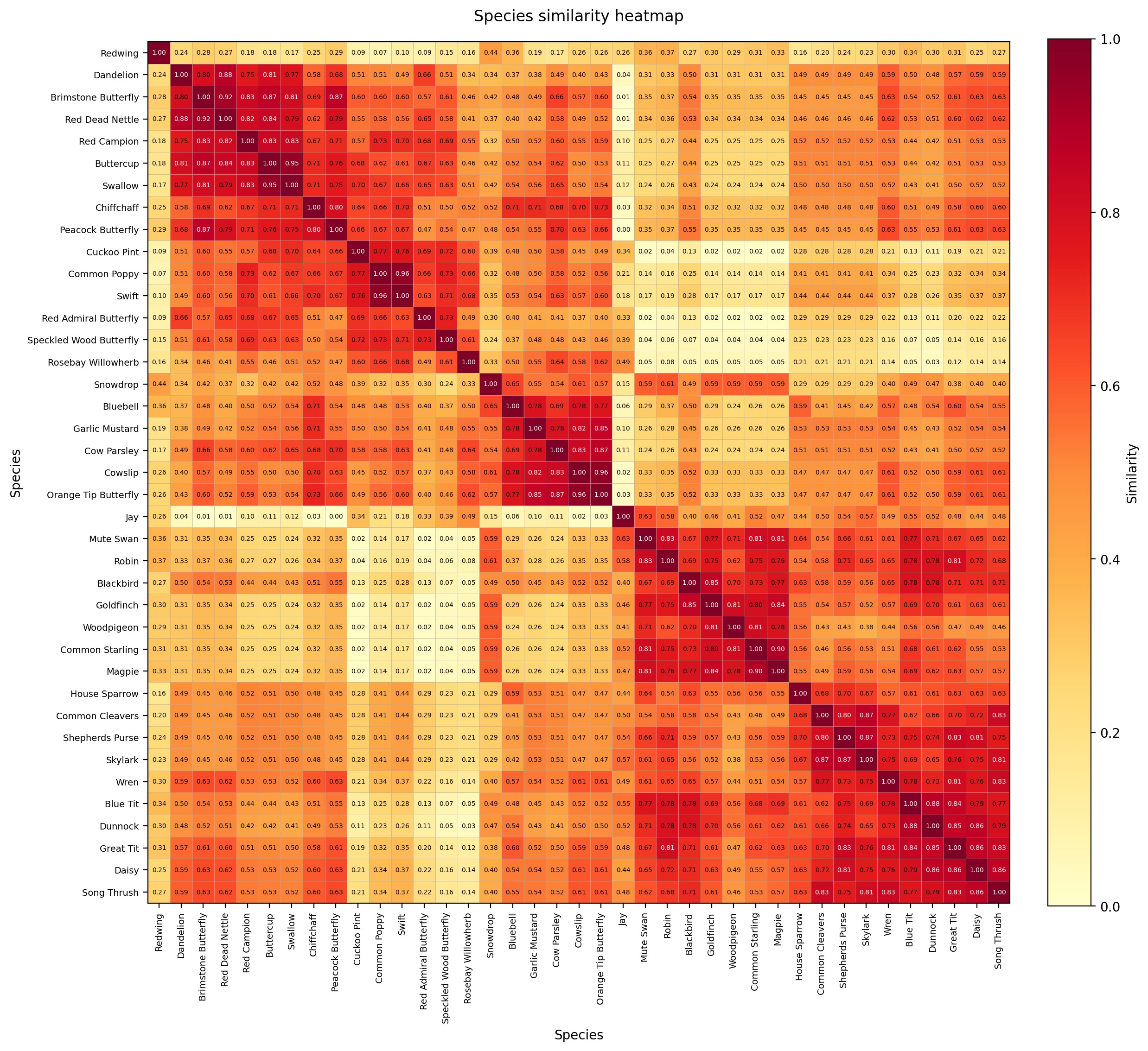
Rather than appearing random, the resulting structure showed several coherent regions:
- Resident bird assemblages
- Spring flowering groups
- Butterfly flight-period clusters
- Summer seasonal communities
- More isolated winter visitor behaviour
Perhaps most interestingly, some of the strongest neighbourhoods crossed traditional taxonomic boundaries entirely and, consequently, the system may be beginning to recover aspects of the seasonal architecture of the year itself.
What the Heatmap Represents
The heatmap should not be interpreted as a map of taxonomy, habitat, or evolutionary relationship.
Instead, it is better understood as a map of seasonal ecological proximity.
Species occupying similar regions of seasonal ecological space appear close together within the matrix.
In many cases this likely reflects:
- Shared environmental forcing
- Similar detectability structure
- Overlapping seasonal windows
- Broad phenological synchrony
At present, the interpretation remains exploratory.
The structure is encouraging, but it is still important not to overstate what the system is doing.
The similarity calculations are ultimately driven by the extracted features and their weighting, and different weighting choices would alter the resulting neighbourhoods.
Nevertheless, the fact that coherent ecological structure emerges at all is encouraging.
If the feature extraction stage were capturing little meaningful information, the resulting matrix would likely appear substantially more chaotic.
A Shift in Perspective
This stage of the work feels like a subtle but important transition. The earlier modelling stages focused on explaining the behaviour of individual species. The newer work begins asking a different kind of question:
“What does the structure of the ecological year itself look like?”
That remains a much larger and more uncertain problem and, for now, the current system is still relatively small, highly simplified, and very much exploratory.
However, it now appears capable of recovering recognisable seasonal neighbourhoods from long-term observational data, while remaining relatively interpretable throughout the process.
That feels like a promising direction.
Next Steps
The current heatmap is only a first visualisation layer.
Several further stages are now possible, including:
- Hierarchical ecological clustering
- Seasonal guild detection
- Community-level seasonality analysis
- Dimensionality-reduction approaches
- Exploration of broader ecological “assemblages”
Whether those structures remain ecologically meaningful as the system grows remains to be seen.
For now, however, the emerging patterns appear interesting enough to justify looking further.
Tool
ODE Solver
A simple tool for exploring time-based models
The seasonal presence and detectability models were developed using a small, general-purpose ordinary differential equation solver, designed for experimentation and visualisation.
It allows simple systems to be defined and explored over time, making it possible to test how patterns might arise from underlying processes.
The application, the models, and instructions on how to run them are provided in the GitHub repository.