
Field Notes Journal Entry
From Signal to Structure
Identifying individual bat calls within a recording and exploring how their timing, shape, and frequency change through a hunting sequence.
In the previous post, I put together a simple, repeatable pipeline for cleaning up bat recordings — reducing background noise and making the underlying signal easier to see.
That alone made a noticeable difference. Calls that were previously buried in noise became clearer, and the overall structure of the recording — the spacing between pulses, and the transition into a feeding buzz — became much easier to interpret.
The next step is to go a little further.
Rather than just looking at the signal, we can begin to identify and measure the individual pulses within it — turning a recording into something more structured, and easier to explore.
From Waveform to Pulses
At its simplest, a bat recording is a sequence of pulses:
- A short, sharp onset
- Followed by a decaying tail
- Repeated over time
The first task is to identify those pulses within the waveform.
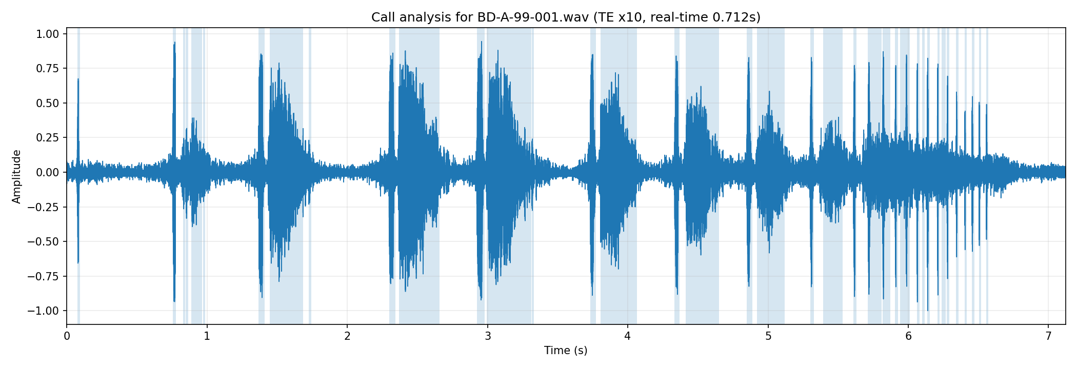
The shaded regions show where individual pulses have been detected. Each region aims to capture both the initial attack and the full decay tail — preserving the natural “conical” shape of the call rather than just the peak and the analysis has successfully identified:
- Individual calls
- Their spacing
- The tightening sequence towards the end
A Simple Workflow
The process of getting from recording to pulse measurements is necessarily iterative:
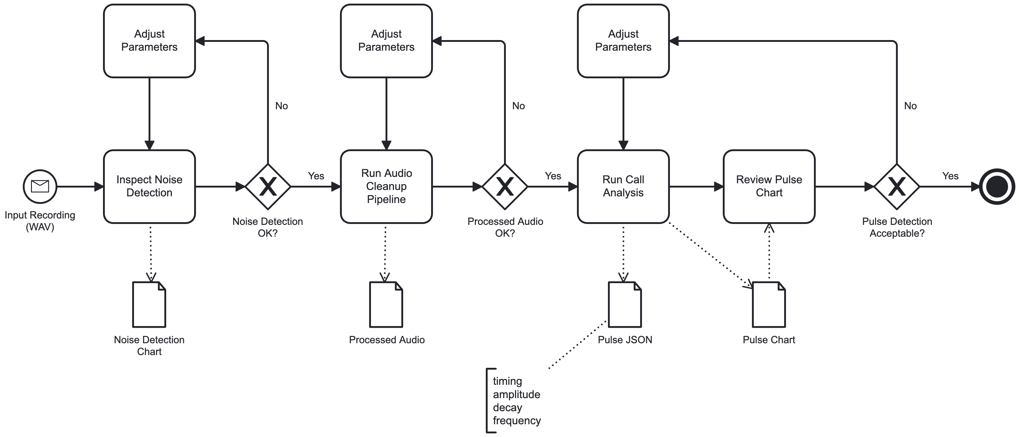
In practice, this comes down to three stages:
- Prepare the signal — reduce noise and make the calls clearer
- Detect pulses — identify where individual calls occur
- Review and refine — check the results and adjust parameters if needed
The aim is not to produce a perfect segmentation, but a consistent and interpretable one.
Inter-Pulse Interval (IPI)
Once pulses are identified, the simplest and most informative measurement is the time between them — the inter-pulse interval (IPI).
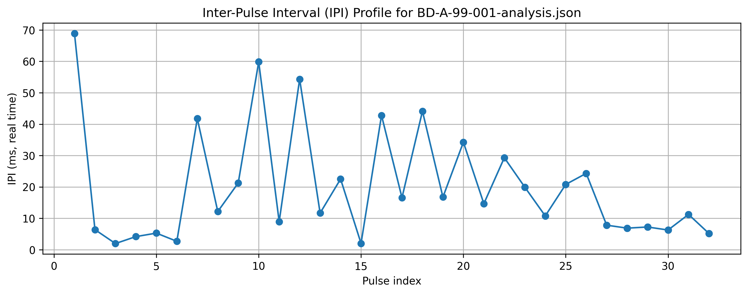
This chart shows how the spacing between calls changes over time.
Three broad phases are visible:
- Search phase — pulses are widely spaced and irregular
- Approach phase — spacing begins to tighten
- Terminal phase (feeding buzz) — pulses become very closely spaced
The final cluster of short intervals is characteristic of a feeding buzz — the rapid sequence of calls a bat produces as it closes in on prey.
This is perhaps the clearest way to “read” a bat pass from a recording.
Frequency Profile
Alongside timing, we can also look at how the frequency of the calls changes.
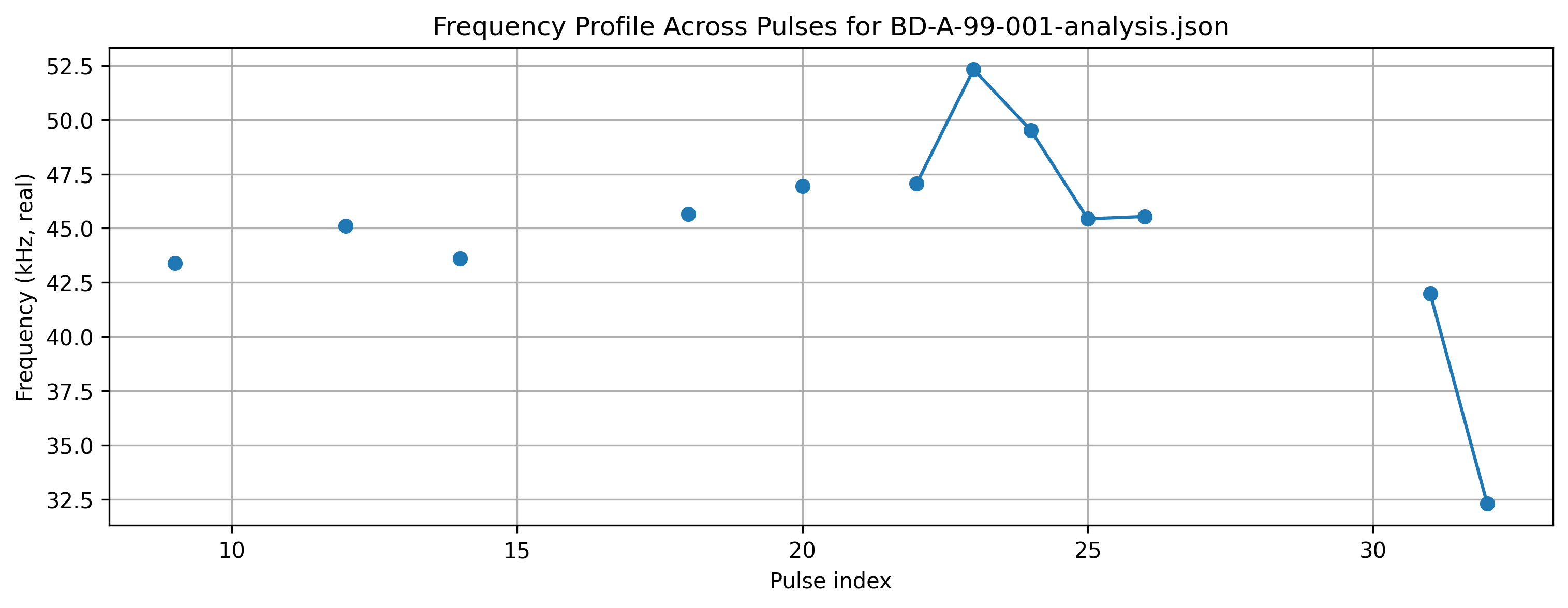
Each point represents a frequency estimate for a pulse where the signal was strong enough to measure reliably.
Most of the calls sit within a relatively narrow band, typical of pipistrelles. Towards the end of the sequence, there is a noticeable drop in frequency.
This is a known feature of pipistrelle calls — the final pulses in the approach can shift downward, which is thought to assist with more precise targeting at close range.
Not every pulse produces a clean frequency estimate, particularly in the dense terminal phase, but the overall pattern is still visible.
Pulse Duration
Another simple measure is the duration of each pulse.
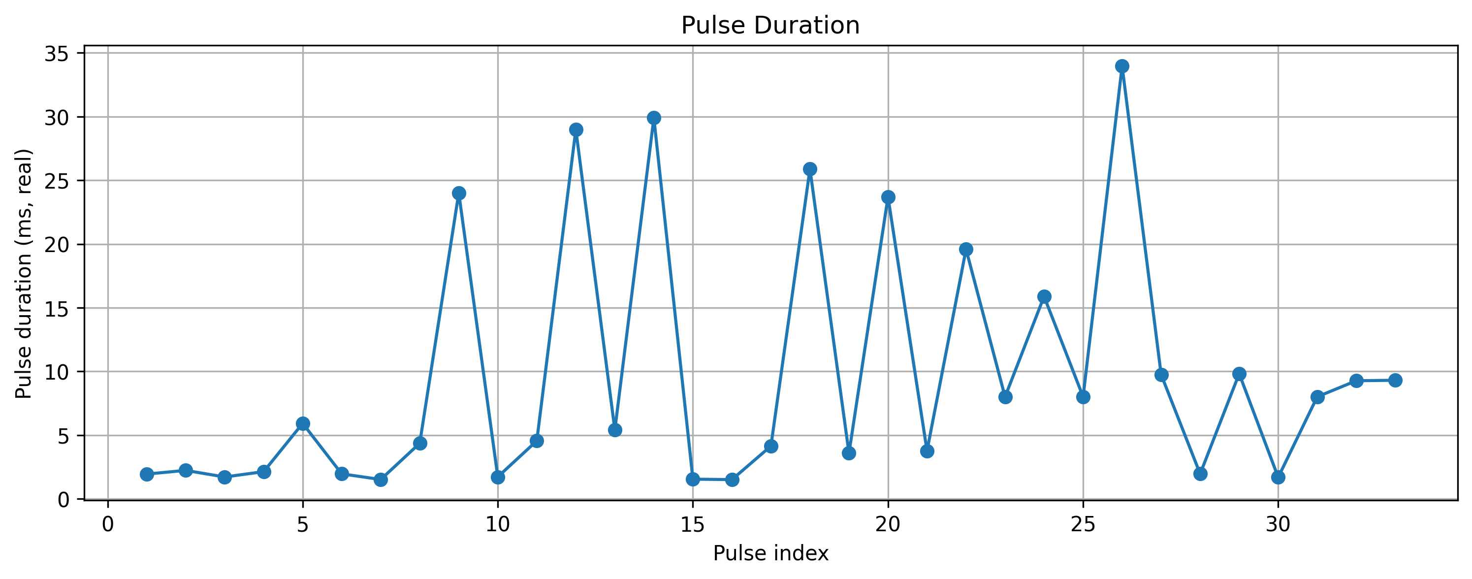
There is some variation throughout the recording, but a general pattern emerges:
- Earlier pulses are often longer and more variable
- Later pulses tend to shorten, particularly in the terminal phase
This reflects the same underlying behaviour as the IPI chart — the bat is increasing the rate at which it samples its surroundings, and the calls themselves become more compact.
Amplitude Profile
Finally, we can look at the amplitude of each pulse.
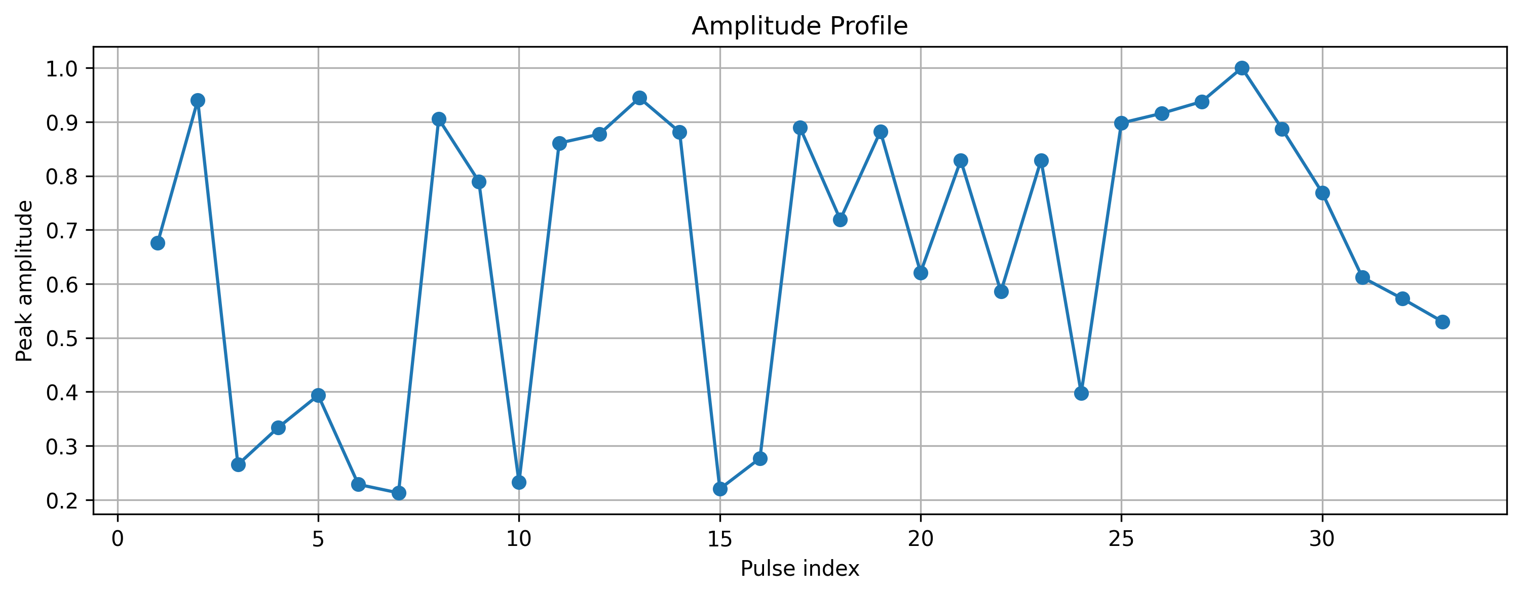
Amplitude is more difficult to interpret directly, as it depends on:
- Distance to the bat
- Direction of the microphone
- Background noise and processing
That said, it still provides useful context:
- Stronger pulses tend to produce more reliable frequency estimates
- Variations can sometimes reflect changes in orientation or proximity
It is best treated as supporting information rather than a primary behavioural indicator.
A Recording Revisited
This recording dates from 1999 — a pipistrelle captured on a time-expansion detector.
At the time, limitations of the affordable recording mechanisms and software available for cleaning the resulting recordings up left them too noisy to be useful for numerical analysis. So it’s particularly pleasing that, now, I’m able to revisit them and apply a more successful cleanup and analysis that clearly shows:
- A sequence of search-phase calls
- A gradual tightening into an approach
- A final, dense cluster of pulses forming a feeding buzz
- A corresponding shift in frequency at the end of the sequence
Nothing new has been added to the recording. The same information was always there.
What has changed is the ability to extract and examine it in a consistent way.
From Recordings to Data
Each recording can now be analysed to yield a set of pulse-level measurements:
- Timing
- Amplitude
- Decay shape
- Frequency
These are written out as structured data (JSON), making it possible to:
- Compare recordings
- Look for patterns across sites or dates
- Revisit older material with the same analysis
In effect, a recording becomes more than a sound — it becomes a small dataset describing a sequence of events.
Closing the Loop
There is something particularly satisfying about returning to these recordings after so many years.
The original observation remains the same — a bat passing overhead on a summer evening — but the tools now allow that moment to be explored in more detail.
What was once a fleeting sound can now be examined, measured, and understood more clearly.
In that sense, this is not just an extension of the processing pipeline, but another step in turning field observations into something that can be revisited and built upon over time.
Spectrogram Viewer and Call Analysis Tool
The spectrogram viewer, audio pipeline, and call analysis implementation are available here:
```