
Field Notes Journal Entry
From Recording to Signal
A simple, repeatable pipeline for turning bat recordings into clearer, more interpretable signals using noise detection, filtering, and spectrogram analysis.
In the previous couple of posts, I returned to some old bat recordings — pipistrelles captured in 1999 — and began exploring them again using a simple spectrogram viewer.
The recordings themselves are often quite noisy. There is background hiss, low-frequency rumble, and a general sense that the signal is “there”, but not always as clearly as it might be. In tools like Audacity, it’s possible to clean this up manually — selecting a noise profile, applying reduction, filtering, and adjusting levels.
What I wanted was something a little more consistent and repeatable: a way of taking a recording and applying the same set of steps each time, producing a result that is easier to interpret while preserving the structure of the original signal.
What follows is a simple pipeline that does exactly that.
Audio Processing Pipeline
The pipeline is designed to make recordings clearer and easier to interpret, while preserving the structure of the original signal.
Overview
Each input recording is processed in the following stages:
| # | Summary | Description |
|---|---|---|
| 1 | Detect noise regions | The recording is scanned to find short sections that are likely to contain background noise only (quiet and low in signal-band energy) - the noise detection algorithm is documented in more detail, below |
| 2 | Build a noise profile | These regions are combined into a single sample, representing the background noise in the recording |
| 3 | Reduce noise (spectral subtraction) | The recording is transformed into the frequency domain, and the estimated noise profile is subtracted from each time slice. A small floor is retained to avoid introducing artefacts |
| 4 | High-pass filter | Low-frequency rumble and handling noise are removed, focusing the signal on the frequency range where bat calls occur (after time expansion) |
| 5 | Normalise | The result is scaled to a consistent peak level, making quiet recordings easier to inspect and listen to |
| 6 | Output | The processed audio is written to disk for further inspection or visualisation |
Design goals
The pipeline is intentionally simple and transparent:
- Repeatable — removes the need for manual selection of noise regions
- Interpretable — each step is easy to understand and adjust
- Non-destructive in spirit — preserves timing and structure of the original signal
- Practical — tuned for real-world field recordings rather than ideal conditions
Notes:
- This is a heuristic workflow, not a studio-grade restoration process
- It works best where recordings contain at least some gaps between calls
- The aim is clarity and consistency, not perfect noise removal
Noise Detection
To reduce background noise automatically, the pipeline includes a simple noise-region detection step. This replaces the manual process of selecting a “quiet” section of audio (as you might do in Audacity).
How It Works
The recording is divided into short, overlapping windows (typically 50 ms). For each window, two measurements are taken:
- Loudness (RMS amplitude) → Quieter windows are more likely to contain background noise only.
- Band energy ratio → The fraction of spectral energy within the expected signal band (for bat recordings, typically ~3.5–6.5 kHz after time expansion).
The band energy ratio is then used to identify the type of signal in the window:
- Low ratio → broadband noise / hiss
- High ratio → structured signal (e.g. bat calls)
A window is considered likely noise if it is both:
- Relatively quiet compared to the rest of the recording, and
- Relatively low in energy within the target band
Thresholds are determined using percentiles, so the detection adapts to each recording rather than relying on fixed values.
From Windows to Regions
Neighbouring “noise” windows are merged into longer regions, and only regions above a minimum duration are kept. These regions are then used as the noise profile for subsequent noise reduction.
Notes and Limitations
- This is a heuristic approach, not a guaranteed classification
- It works best when recordings contain genuine gaps between calls
- On dense or noisy recordings, it will tend to select the least signal-like sections rather than perfectly clean noise
- The goal is consistency and practicality, not perfect isolation
Bringing it Together
This pipeline provides a clearer view of the original signal while preserving it’s structure:
- The timing of calls
- The spacing between them
- The transition into feeding buzz
What changes is simply the clarity with which those features can be seen and heard. This is quite clear from the two spectrograms, below:
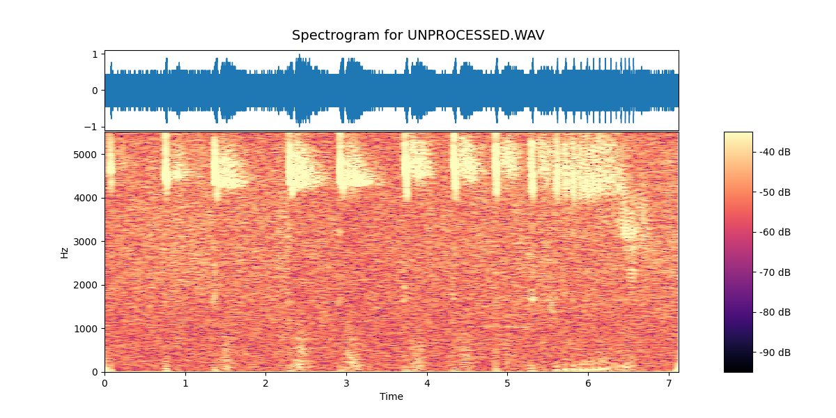
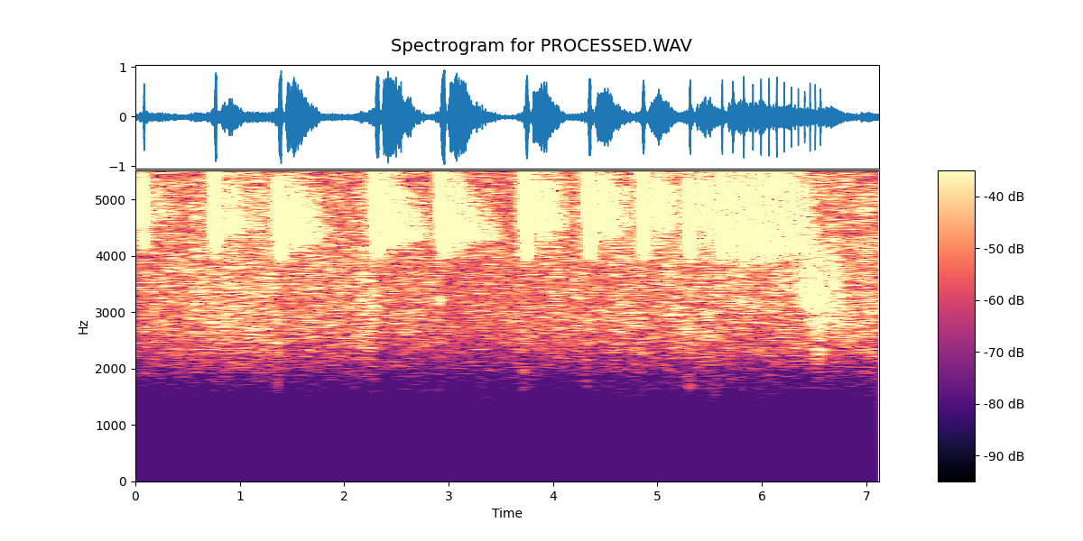
In the unprocessed recording, the signal is present but sits within a broad background of noise. The spectrogram shows a continuous haze across much of the frequency range, and the individual calls are less clearly defined against it.
In the processed version, that background is reduced, and the structure of the calls stands out much more distinctly. The individual pulses are clearer, the spacing between them is easier to follow, and the transition into the feeding buzz is more obvious.
Nothing new has been added to the signal — the same information is there in both cases — but the processing makes it far easier to see what is happening.
In practice, this makes a significant difference. A recording that might previously have required careful listening and interpretation becomes something that can be inspected visually and understood more directly.
A Small Step Towards Consistency
Undoubtedly the most useful aspect of the pipeline is that it is repeatable.
Rather than manually selecting noise regions and adjusting settings each time, the same process can be applied across recordings — whether they were made yesterday or, as in this case, over twenty-five years ago.
That opens up the possibility of treating these recordings not just as isolated observations, but as part of a longer sequence: something that can be compared, revisited, and built upon over time.
Next Steps
With the processing in place, the focus shifts back to the field.
New recordings can now be captured, processed, and visualised in a consistent way, making it easier to explore patterns in behaviour — and to relate what is heard in the moment to what can be seen afterwards.
In that sense, this becomes another layer of the Field Notes Journal: a way of turning sound into something that can be observed, compared, and understood.
Field Note — Spectrogram Viewer and Audio Pipeline Implementation
The spectrogram viewer and audio pipeline processor is available here:
→ View the spectrogram viewer and pipeline processor on GitHub