
Winter Visitor Model
Some species are present only during the winter months. They arrive in autumn, persist through winter, and depart again in spring — their period of presence spanning the end and beginning of the year.
This model describes that pattern: a seasonal presence that wraps around the year boundary, with a winter peak and near-absence through summer.
Concept
This model describes species that are present during the winter months, with activity spanning the end and beginning of the year.
It answers the question:
When is the species present?
Like the seasonal model, presence is limited to part of the year. Unlike it, the active period crosses the year boundary.
The model defines a seasonal target, representing expected activity through the year. The observed signal then adjusts towards this target over time.
The target combines:
- A winter component, representing peak presence
- An optional autumn component, representing arrival
- A summer suppression, reducing activity during the off-season
Together, these produce a cycle that rises through autumn, peaks in winter, and falls away into spring.
Model Parameters
A small number of parameters control the behaviour of the model:
| Parameter | Purpose |
|---|---|
| INITIAL_Y | Sets the starting value of the modelled signal |
| BASELINE | Sets any persistent background level (typically near zero for winter visitors) |
| WINTER_WEIGHT | Controls the strength of the winter peak |
| AUTUMN_WEIGHT | Controls the strength of the autumn arrival phase |
| SUMMER_DIP | Controls the strength of the summer suppression |
| WINTER_PEAK | Sets the timing of peak winter presence |
| AUTUMN_PEAK | Sets the timing of autumn arrival |
| SUMMER_LOW | Sets the timing of lowest summer activity |
| WINTER_WIDTH | Controls how concentrated the winter peak is |
| AUTUMN_WIDTH | Controls the breadth of the arrival phase |
| SUMMER_WIDTH | Controls the breadth of the summer low |
| GROWTH_RATE | Controls how quickly activity rises towards the seasonal target |
| DECAY_RATE | Controls how quickly activity declines |
Together, these parameters define:
- When the species arrives and peaks
- How concentrated the winter period is
- How gradually or abruptly the species appears and disappears
- How strongly the species is absent through summer
All timing parameters are expressed in months on a circular 12-month scale.
Mathematical Form
The model is a first-order system:
dy/dt = rate × (target(t) - y)
Where:
- y(t) is a relative, dimensionless measure of observable activity
- target(t) is the seasonal activity target
- rate is selected using GROWTH_RATE or DECAY_RATE depending on whether the signal is rising or falling
The target function is constructed from smooth periodic components:
target(t) = winter(t) + autumn(t) - summer(t) + BASELINE
Each component is a smooth function over a 12-month cycle, allowing continuous variation without discontinuities.
Model Behaviour
When applied over a full year, the model produces a winter-centred cycle:
- Activity rises through autumn as the species arrives
- Peaks in mid-winter
- Declines through late winter and early spring
- Remains close to zero through summer
The shape depends on:
- The timing and strength of the winter and autumn components
- The breadth of the winter peak
- The strength of summer suppression
- The rate at which the system responds to change
Unlike the seasonal presence model, the season is not bounded within a single part of the calendar year. Instead, it wraps across the year boundary.
Fitting to Observations
The model can be fitted to observed monthly data.
A parameter fitting process:
- Infers a plausible seasonal structure from the data
- Generates candidate parameter sets
- Runs the model
- Compares simulated and observed curves
- Scores the match
- Repeats to identify good solutions
This produces a set of parameters that describe the species’ seasonal behaviour.
These parameters are broadly interpretable:
- WINTER_PEAK → timing of peak presence
- AUTUMN_PEAK → timing of arrival
- WINTER_WIDTH → concentration of winter activity
- AUTUMN_WIDTH → spread of the arrival phase
- SUMMER_DIP / SUMMER_LOW → strength and timing of absence
Together, they provide a compact description of a species’ winter pattern.
As with the other models:
- Parameters are estimates rather than exact values
- Different combinations may produce similar curves
- Interpretation is most reliable when considered alongside the fitted curve
Normalisation
Model outputs are expressed as a relative measure of activity.
To allow comparison across species, results are normalised so that:
- 1.0 → peak activity
- 0.5 → half of peak activity
- 0.0 → effectively zero
This focuses attention on the timing and shape of seasonal variation.
Example
Redwing
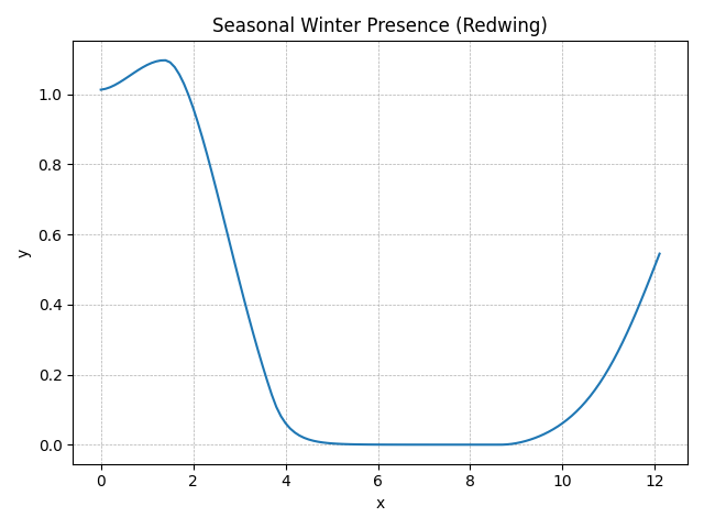
Observed data show:
- Arrival in autumn
- A peak through mid-winter
- Departure in spring
- Absence through summer
The fitted model describes this pattern using:
- A winter peak centred early in the year
- A weaker autumn component representing arrival
- Strong summer suppression, reducing activity to near zero
The resulting curve captures:
- A seasonal cycle that wraps across the year boundary
- A concentrated winter presence with extended absence
Seasonal signature (modelled):
- Presence: November/December–March
- Peak: December–January
- Width: moderate
- Decline / absence: strong summer absence, with little residual activity
Interpretation
This model represents species that are present only during the winter period, with activity spanning the year boundary.
It provides a minimal explanation for patterns seen in the Seasonal Analyses, showing that a small number of simple processes can produce:
- Winter-centred presence
- Distinct arrival phases
- Extended absence through summer
The model does not attempt to describe detailed ecological mechanisms. Instead, it offers a way of understanding how seasonal structure and timing combine to produce the observed patterns.
In Context
Within the broader modelling framework, this model corresponds to species that are:
- Absent for much of the year
- Present across the year boundary
- Peaking in winter
These contrast with:
- Seasonal presence species, active within a bounded window
- Resident species, present throughout the year but variably detectable
Together, these models describe three distinct ways in which species occupy the year.
Tool
ODE Solver
A simple tool for exploring time-based models
The models presented here were developed using a small, general-purpose ordinary differential equation solver, designed for experimentation and visualisation.
It allows simple systems to be defined and explored over time, making it possible to test how patterns might arise from underlying processes.
The application, the models, and instructions on how to run them are provided in the GitHub repository.