
Seasonal Presence Model
Some species occupy only part of the year. They appear, persist for a time, and then disappear again — not because they are absent from the wider world, but because they are no longer visible in this place.
This model describes that pattern: a seasonal presence that rises within a defined window and declines outside it.
Concept
The model combines three simple elements:
- A seasonal driver, representing environmental change through the year
- A seasonal window, limiting when presence is possible
- A decay term, allowing activity to fall away outside the active period
Together, these produce a curve that rises into a season, reaches a peak, and then declines again.
The result is not a prediction of abundance, but a simplified representation of when a species is observable, and how sharply that observation begins and ends.
Model Parameters
A small number of parameters control the behaviour of the model:
| Parameter | Purpose |
|---|---|
| GROWTH | Controls how strongly seasonal conditions drive the appearance of the species. Higher values produce a more rapid rise and a more pronounced peak |
| DECAY | Controls how quickly activity declines during the active period. Lower values allow activity to persist; higher values lead to a shorter, more sharply defined season |
| OOS_DECAY | Increases the rate of decline outside the seasonal window. This term ensures that activity falls away rapidly once the species is no longer present, rather than lingering artificially |
Together, these parameters define the balance between emergence, persistence, and disappearance, shaping both the timing and sharpness of the seasonal pulse.
Mathematical form
The model is expressed as a first-order ordinary differential equation:
dy/dt = GROWTH * S(t) * W(t) - decay(t) * y
Where:
- y(t) is a relative, dimensionless measure of observable activity
- S(t) is a smooth seasonal forcing function
- W(t) is a seasonal window, constraining when presence is possible
- decay(t) controls how rapidly activity declines, particularly outside the active period
The seasonal forcing - S(t) - is represented as a smooth annual cycle, scaled between 0 and 1:
S(t) = (1 + cos(2π(t - peak)/12)) / 2
The seasonal window W(t) is constructed from two logistic functions, representing the onset and end of the active period:
W(t) = rise(t) × fall(t)
with:
rise(t) = 1 / (1 + exp(-k(t - start)))
fall(t) = 1 / (1 + exp(k(t - end)))
Outside the seasonal window, the decay term increases, causing activity to fall more rapidly:
decay(t) = DECAY + OOS_DECAY × (1 - W(t))
Model behaviour
When applied over a full year, the model produces a single seasonal pulse:
- activity begins gradually as conditions become favourable
- reaches a peak within the active period
- and then declines, often more rapidly, once the season ends
The timing and shape of this pulse depend on a small number of parameters:
- the position and strength of the seasonal driver
- the start and end of the seasonal window
- and the rate at which activity decays outside that window
By adjusting these, the model can represent a range of seasonal behaviours, from brief and sharply bounded appearances to more extended periods of activity.
Examples
Bluebell
The bluebell provides a clear example of a strongly seasonal species.
Observed data show a narrow window of occurrence, with a rapid rise in spring, a short peak, and a swift decline after flowering.
The model reproduces this pattern using:
- A tightly constrained seasonal window
- Relatively strong decay outside the active period
- A seasonal driver aligned with spring conditions
Model simulation (Seasonal Presence Model)
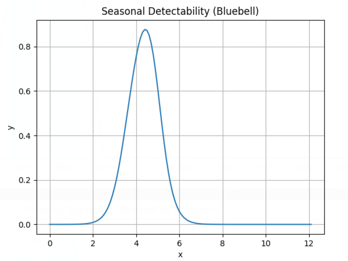
The resulting curve captures the brevity and timing of the bluebell season, reflecting the way in which the species appears briefly and then recedes from view.
Swift
The swift represents a different form of seasonal presence, driven by migration rather than growth or flowering.
Observed data show:
- A rapid arrival in late spring
- A concentrated period of activity through summer
- A swift departure
The model reproduces this pattern with:
- A narrow seasonal window
- Strong out-of-season decay
- A forcing function aligned with summer conditions
Model simulation (Seasonal Presence Model)
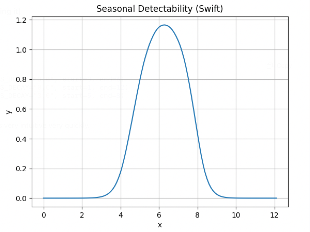
The resulting curve reflects the sharply bounded period during which swifts are present, and their rapid disappearance from the local landscape.
Interpretation
This model is intended to represent species whose presence is seasonally constrained — those that are only observable during a particular phase of their life cycle or migration.
It is deliberately simple and abstract — closer to a minimal representation than a description of detailed ecological mechanisms — and is intended to explore whether the observed patterns can arise from a small number of underlying processes, not to predict observations.
It provides a minimal explanation for patterns seen in the Seasonal Analyses, showing that a small number of simple processes are sufficient to produce:
- Sharply bounded flowering periods
- Migration-driven appearances
- Other forms of seasonal presence
The model does not attempt to describe the underlying biological mechanisms in detail. Instead, it offers a way of understanding how the observed patterns might arise from the interaction of seasonal forcing, limited availability, and decline.
In Context
Within the broader set of observations, this model corresponds to species that are:
- Absent for part of the year
- Present within a defined seasonal window
- Often sharply bounded in time
These contrast with species that are always present but vary in detectability — a pattern described by the Resident Detectability Model.
Reference
The JSON-format ODE Solver simulation files used to generate these models — including parameter values and the defining equations — are available for download in the reference section.
These provide the exact configurations used to produce the example curves shown here.