
Resident Detectability Model
Some species are present throughout the year. They do not appear and disappear, but remain a constant part of the landscape — their visibility changing with season, behaviour, and context.
This model describes that pattern: a continuous presence in which detectability rises and falls through the year without ever reaching zero.
Concept
The model assumes that a species is always present, and that what changes over time is not presence, but how readily it is observed.
Rather than generating activity within a seasonal window, the model defines a seasonal target, representing expected detectability at a given point in the year. The observed signal then adjusts towards this target over time.
The target itself combines several simple elements:
- A baseline level, representing persistent year-round presence
- A winter / early-spring peak, reflecting increased visibility or activity
- An autumn / early-winter recovery, as detectability rises again
- A summer dip, when activity or visibility is reduced
Together, these produce a continuous annual cycle with characteristic peaks and troughs, but no enforced absence.
Model Parameters
A small number of parameters control the behaviour of the model:
| Parameter | Purpose |
|---|---|
| BASELINE | Sets the minimum year-round detectability, representing continuous presence |
| WINTER_WEIGHT, AUTUMN_WEIGHT, SUMMER_DIP | Control the relative strength of seasonal features, shaping the prominence of peaks and troughs |
| *_PEAK | Determine the timing of seasonal features within the year |
| *_WIDTH | Control the breadth of peaks and dips, from gradual variation to more concentrated periods |
| RESPONSE_RATE | Controls how quickly the observed signal adjusts to changes in the seasonal target |
| GROWTH_RATE / DECAY_RATE (if used) | Allow asymmetric dynamics, for example faster decline in summer and slower recovery towards winter |
Together, these parameters define the balance between persistence and variation, shaping the timing and form of the annual cycle.
Mathematical form
The model can be written as:
dy/dt = RESPONSE_RATE × (target(t) - y)
Where:
- y(t) is a relative, dimensionless measure of observable activity
- target(t) is the seasonal detectability target
- RESPONSE_RATE controls how quickly the system responds
The target function is constructed from smooth annual components:
target(t) = BASELINE + winter(t) + autumn(t) - summer(t)
Each component is represented as a raised cosine function:
component(t) = (1 + cos(2π(t - peak)/12)) / 2
with an exponent controlling its width.
Together, these components produce a continuous, periodic function describing expected detectability across the year.
Model behaviour
When applied over a full year, the model produces a smooth, continuous cycle:
- detectability rises into a winter or early-spring peak
- declines through the summer months
- and recovers again towards autumn and winter
Unlike the seasonal presence model, the signal does not collapse to zero. Instead, it fluctuates around a persistent baseline, reflecting continuous presence.
The shape of the curve depends on:
- the timing and strength of seasonal components
- the relative depth of the summer dip
- and the rate at which the system responds to change
By adjusting these, the model can represent a range of resident behaviours, from relatively stable presence to strongly varying detectability.
Example
Robin
The robin provides a clear example of a resident species with seasonal variation in detectability.
Observed data show:
- high visibility in winter and early spring
- a reduction through summer
- and a gradual recovery towards the end of the year
The model reproduces this pattern using:
- a persistent baseline
- a winter / early-spring peak
- a summer dip
- and an autumn recovery
Model simulation (Resident Detectability Model)
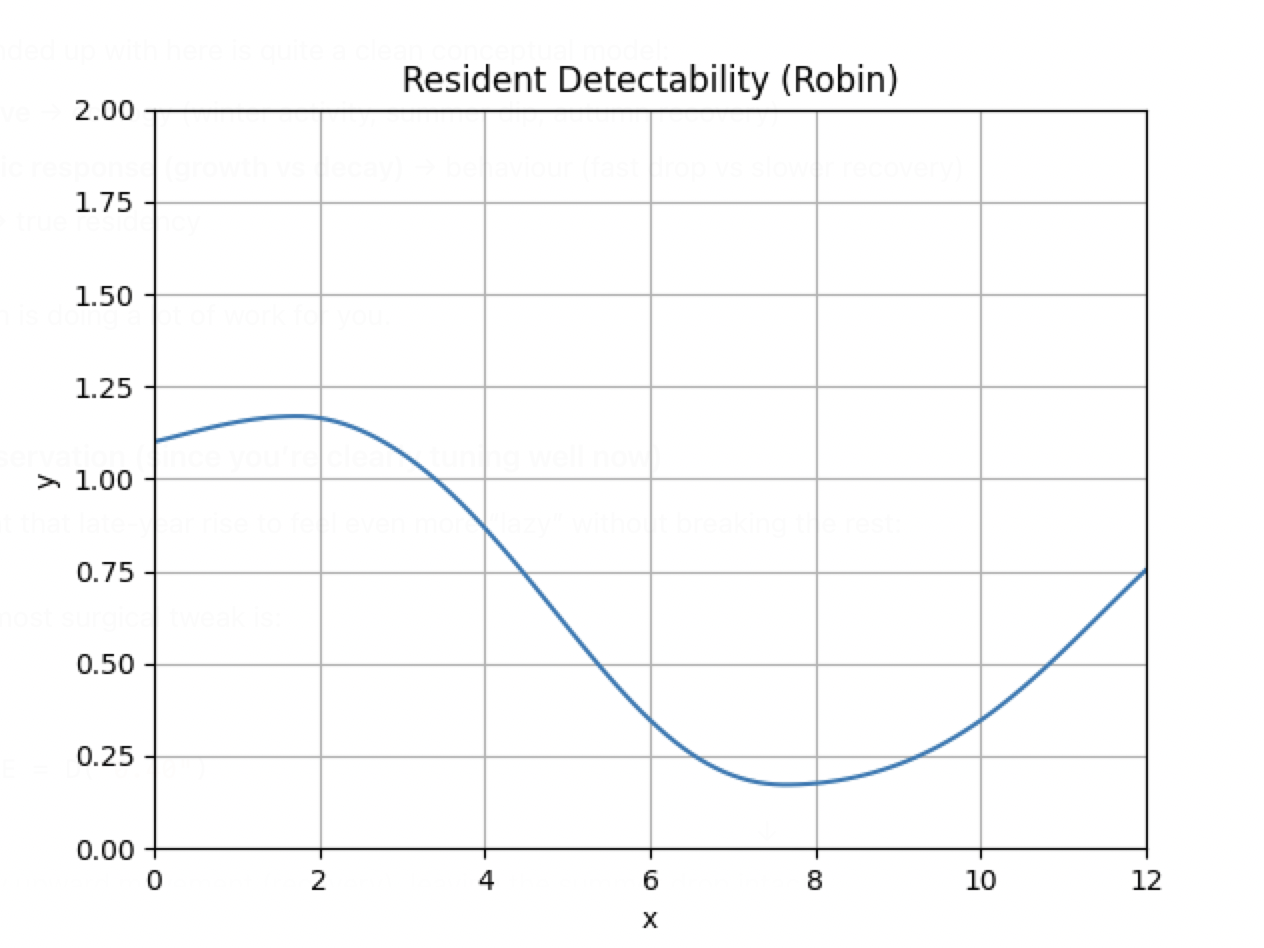
The resulting curve captures the continuous presence of the species, while reflecting changes in behaviour and visibility through the year.
Interpretation
This model is intended to represent species that are always present but variably detectable.
It is deliberately simple and abstract — closer to a minimal representation than a description of detailed ecological mechanisms — and is intended to explore whether the observed patterns can arise from a small number of underlying processes, not to predict observations.
It provides a minimal explanation for patterns seen in the Seasonal Analyses, showing that variation in observation does not necessarily imply absence, but can arise from:
- Behavioural change
- Seasonal activity patterns
- Variation in visibility
The model does not attempt to describe the underlying biological mechanisms in detail. Instead, it offers a way of understanding how continuous presence combined with seasonal variation can produce the observed patterns.
In Context
Within the broader set of observations, this model corresponds to species that are:
- Present throughout the year
- Never fully absent
- Varying primarily in detectability rather than occurrence
These contrast with species that are only present for part of the year — a pattern described by the Seasonal Presence Model.
Reference
The JSON-format ODE Solver simulation files used to generate these models — including parameter values and the defining equations — are available for download in the reference section.
These provide the exact configurations used to produce the example curves shown here.